Introduction/Background

51 Pegasi b, the first exoplanet discovered around a main-sequence star in 1995 [1], surprised astronomers because it's a planet that does not look like any planet in our solar system. People call it a "hot Jupiter", based on its orbital period and mass. This is not the only exotic exoplanet people have found. Since then, approximately 6,000 exoplanets [2] have been discovered, and many of them still lack counterparts to our solar system's planets. The "period, mass" classification scheme is straightforward, but it only accounts for two features of the planets. Until today, no standardized exoplanet classification scheme has been widely accepted. Therefore, we want to use unsupervised ML to create a standardized classification algorithm for exoplanets.

The main dataset we will use is the Kepler Objects of Interest (KOI) table. It is built on planet transit data from the Kepler telescope. The KOI database is a good start for our unsupervised learning.

It is also notable that the KOI dataset has classified planets as confirmed, candidate, and false positive. This is where we want the supervised learning model to work on. There has been extensive work on using ML, including CNNs and transformers[3][4], to identify false positives. We aim to reproduce and improve on these results.

Dataset Links

• Kepler data products overview
• Kepler Objects of Interest (KOI) table
• Exoplanet archive

Problem Definition

How to use ML to discover subgroups of exoplanets? How can ML help identify more exoplanet candidates or false positives? The confirmation of exoplanets, and also the classification of exoplanets, has long been a subjective and case-by-case job. This calls for the use of ML algorithms to group planets by statistics when little physics prior knowledge can be provided, and identify false positives when subsequent observations are not yet available.

Methods

1 Supervised Machine Learning

1.1 Data Preprocessing

Based on the work by Rafaih, Murray et al.[4], we selected eight features for our training model, which are koi_period, koi_impact, koi_duration, koi_depth, koi_model_snr, koi_bin_oedp_sig, koi_steff, and koi_srad. These features are selected for their physical interpretability and their representation of low-level planetary parameters. The predicted feature is koi_pdisposition, which includes two categories: CANDIDATE and FALSE POSITIVE.

Feature	Description
koi_period	Represents the orbital period (days) of the potential exoplanet — the interval between consecutive planetary transits.
koi_impact	Calculated impact parameter, measuring the perpendicular distance between the center of the star and the planet’s orbit.
koi_duration	Duration (hours) from the planet’s first contact with the star until the last contact during transit.
koi_depth	Fractional decrease in the star’s brightness during a planetary transit.
koi_model_snr	Transit signal-to-noise ratio, representing the strength of the observed transit signal.
koi_bin_oedp_sig	Significance of the difference between odd and even transit depths in binned data.
koi_steff	Star’s effective temperature (Kelvin).
koi_srad	Star’s radius (in solar radii).

The raw dataset has 9564 rows. Among the eight selected features, koi_bin_oedp_sig has the highest percentage of missing values, approximately 16%. The features koi_impact, koi_depth, koi_model_snr, koi_steff, and koi_srad each have around 3.8% missing values. After experimentation, we decided to drop the missing values rather than input the missing because: a). exoplanet detection requires high precision and reliability, and b). a small imputation bias could introduce significant distortions. Therefore, we remove all records having missing values. The final dataset has 7995 rows, which are ready for model training and testing.

We split the dataset into 80% for training and 20% for testing. Before training the model we applied Min-Max Scaling to normalize all features to a range between 0 and 1. Min-Max Scaling can prevent the models from being overly sensitive to large feature scales. Also, it can support faster and more stable model convergence during the training process.

In terms of evaluation metrics, we focus on precision and recall score for evaluating our supervised machine learning models. Since our positive class is false positive exoplanets, precision tells us among all exoplanets predicated false positives, how many are truly false positives. Recall tells us among all the actual false positive exoplanets, how many are successfully identified. Both of the precision and recall scores are important to our study. To balance these two objectives, we also consider the F1 score, which combines precision and recall into a single metric.

Accuracy might not be the best evaluation metric since our priority is to find false positive exoplanets . A model might have high accuracy, but it gives the equal importance of both false positive and candidate exoplanets. However, our study focuses more on the false positive exoplanets given the objective of reducing the time and resources spent investigating non-real exoplanets.

1.2 Algorithm #1 - Logistic Regression

We tested the Logistic Regression algorithm as one of our baseline models for supervised machine learning classification. Logistic Regression is a well-established statistical model that estimates the probability of a binary outcome using a logistic (sigmoid) function. It serves as a simple yet powerful model that provides interpretability through its coefficients, which directly indicate the influence of each feature on the target variable.

Initially, we selected Logistic Regression because of its efficiency, interpretability, and strong performance on linearly separable datasets. It also serves as an excellent benchmark before exploring more complex models such as ensemble methods. Moreover, Logistic Regression supports regularization techniques, which help prevent overfitting and improve generalization performance.

1.2.1 Model Implementation

The Logistic Regression model works by finding the parameters for each feature to minimize the loss function using optimization process. The model uses a linear combination of input features through the sigmoid function to produce probabilities between 0 and 1, to classify into binary categories.

We used the Logistic Regression implementation with the default parameters as a baseline model. Based on this initial performance, we performed hyperparameter tuning using GridSearchCV to explore different configurations of key parameters like penalty type (L1 and L2), solver (e.g., liblinear, lbfgs, saga) and regularization strength (C).

We conducted a 5-fold cross-validation during the grid search process to select the optimal combination of hyperparameters based on the ROC-AUC score, which measures the model’s ability to distinguish between classes.

After identifying the best hyperparameters, we retrained the best-performing Logistic Regression model on the full training set and evaluated it on the test set. The performance metrics ( precision, recall, F1-score, and ROC-AUC), were analyzed to assess the final model's prediction. Additionally, this model also provides a list of important features that strongly influence the outcome. This interpretability is one of Logistic Regression’s primary advantages compared to more complex models.

1.2.2 Result and Discussion

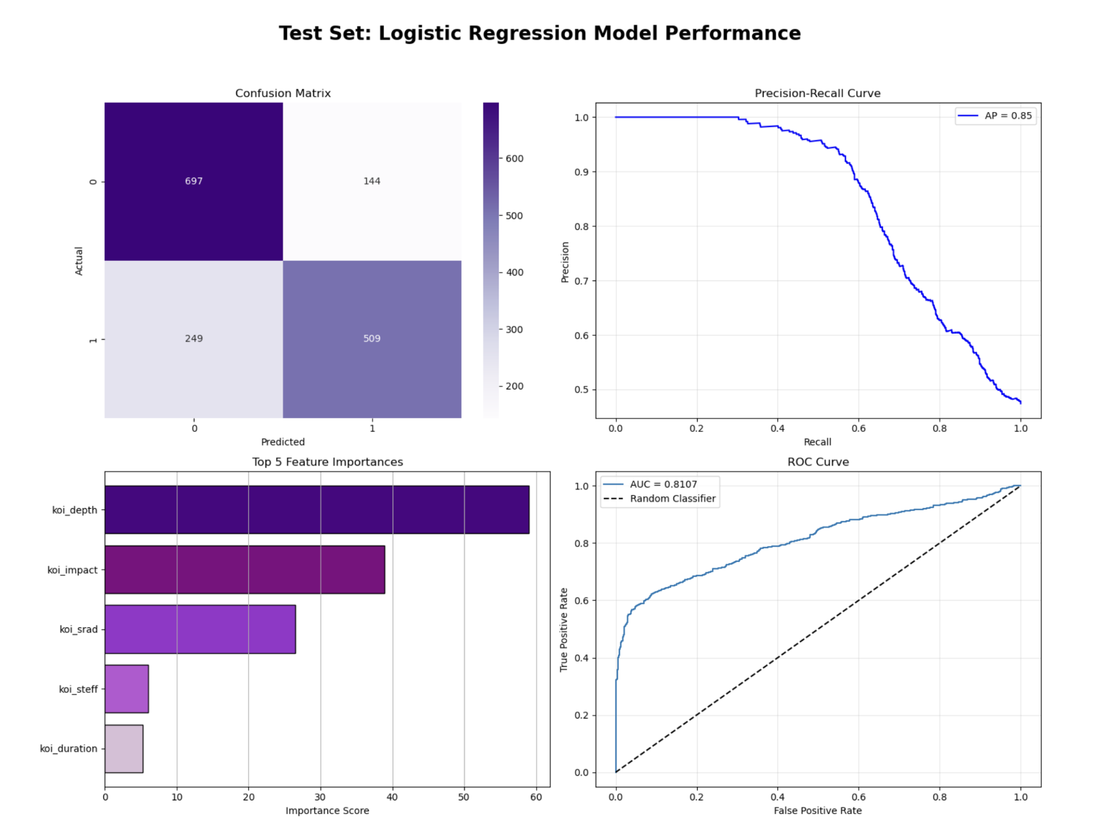
In our study, identifying false positive exoplanets is the primary objective, as misclassifying them as candidate exoplanets can lead to wasted research efforts. Therefore, we prioritized metrics that emphasize the balance between positive predictions and true outcomes — specifically, Precision, Recall.

When trained with default hyperparameters, the Logistic Regression model achieved a Precision of 0.84, Recall of 0.55, Average Precision of 0.82 and ROC_AUC of 0.79. These results indicate that while the model was effective at correctly identifying false positive cases, it struggled to capture all actual false positives. It can be due to insufficient regularization control.

To improve model performance, we conducted hyperparameter tuning using GridSearchCV, using various regularization strength (C), penalty type (L1, L2), and solver methods. When precision was used as the scoring metric, the tuned model achieved a Precision of 0.97, Recall of 0.24, Average Precision of 0.69, and ROC-AUC of 0.61, a decline in overall performance compared to the default configuration. This happened because optimizing strictly for precision hence classifying fewer false positives and thus missing many true cases.

When we changed the scoring metric to roc_auc, the model achieved a much better balance, with Precision of 0.78, Recall of 0.67, Average Precision of 0.85, and ROC-AUC of 0.81. The best-performing configuration corresponded to L1 regularization, liblinear solver, and C = 100. This setup improved the model’s Recall from 55% to 67%, F1-score from 67.3% to 72%, and ROC-AUC from 0.79 to 0.81.

The improvements can be attributed to the L1 penalty, where less important features are ignored and improving generalization. From the Precision–Recall and ROC curves, the tuned model achieved an average precision of 0.85 and an AUC of 0.81, confirming that it maintains a strong discriminative ability between the two classes. The top five features identified by the model are koi_depth, koi_impact, koi_srad, koi_steff and koi_duration.

While the optimized Logistic Regression model demonstrates solid performance, the moderate recall suggests that there may still be complex nonlinear relationships in the data that linear models cannot capture. Therefore, more sophisticated models need to be explored.

1.3 Algorithm #2 - XGBoost

We tested the XGBoost algorithm since it is an ensemble learning method that combines multiple weak models to form a stronger model. XGBoost uses decision trees as the base learners, which aligns with our original plan to test a single Decision Tree algorithm for supervised machine learning. We transitioned from a single Decision Tree to XGBoost because we found that XGBoost provides greater predictive results. Also, XGBoost has the same capability of revealing feature importance like Decision Tree.

1.3.1 Model Implementation

How the XGBoost algorithm works can be explained as follows. It first constructs a simple decision tree, and each subsequent tree is trained on the errors of the previous tree. Through this iterative process, each tree learns from the mistakes of the previous trees, so the ensemble keeps improving. As a result, XGBoost usually can have more accurate and robust predictions.

We use the XGBClassifier from scikit-learn. The default hyperparameters include a tree-based booster (gbtree), a binary:logistic as the objective function, and default learning rate with 0.3. We first train the default model as a baseline. Based on that baseline, we performed hyperparameter tuning to observe if the model’s performance can be improved. We use GridSearchCV to search for the best hyperparameter combinations. We have a focus search on the following parameters, including learning rate, n_estimators, max_depth, min_child_weight, reg_alpha (L1 regularization), and reg_lambda (L2 regularization).

We also use five-fold cross-validation during the grid search process. By doing so, we want to find the most reliable and robust parameters for XGBoost. After having the best model parameters, we re-evaluate the best model with cross-validation to verify its consistency before testing. Once we are satisfied with the validation result, we apply the model to the test set to obtain the final evaluation of the best-performing XGBoost model.

1.3.2 Result and Discussion

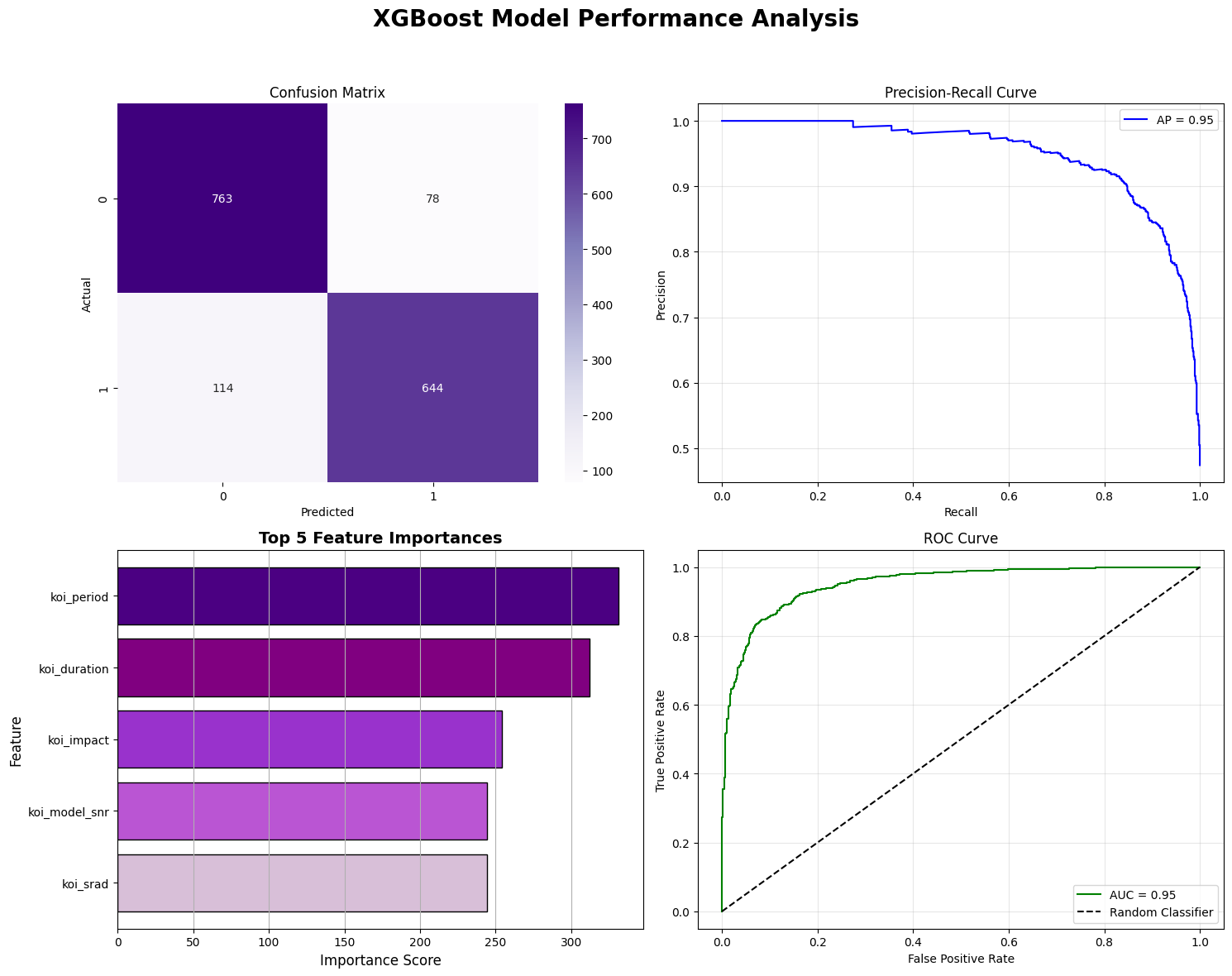
Across our experiments, XGBoost demonstrated consistently strong performance for false positive exoplanet detection. With default hyperparameters, the model already achieved high performance, with 88% precision, 85% recall, and 86% F1 score, which outperforms a logistic regression. After hyperparameter optimization, precision further improved to 89% and 87% F1 score. This result indicates that XGBoost is able to preserve a strong balance between precision and recall.

The top five features identified by XGBoost are koi_period, koi_duration, koi_impact, koi_model_snr, and koi_srad. These features have clear physical interpretations, including orbital activity, the perpendicular distance between the stellar center and the planet’s trajectory, and the signal-to-noise ratio and stellar radius. The XGBoost algorithm demonstrates its strong ability to classify false positives by using only foundational physical observational data.

By reading the Precision–Recall and ROC curves, we found that the XGBoost model achieves an average precision of 0.95 and an AUC of 0.95. These metrics confirm that our model maintains high prediction ability.

For the next steps, we will apply neural networks and explore additional features to observe whether we can improve the model’s performance in identifying false positive exoplanets.

2 Unsupervised Machine Learning

2.1 Data Preprocessing

Though we have proposed to use the Kepler dataset for classifying exoplanets, it was found to be improper for this mission, because it lacks a variety of exoplanets. Kepler only measures the transiting planets, meaning that it has a strong preference for close-in planets. Therefore, not many planet clusters can be found using the pure Kepler dataset. We decided to use the Exoplanet Archive, which is also listed in the proposal.

We first choose proper features from the dataset for clustering exoplanets. Considering that many features are incomplete, we choose the most complete and also the most important features for exoplanets, which are the planet orbital period (pl_orbper), planet radius (pl_rade), and planet mass (pl_bmasse). We then drop all the data without any of the three features. This brings our dataset size from 6007 rows to 1415 rows. This large dataset size reduction might bring worries about whether the smaller dataset can represent the original dataset. Considering that all three parameters are important to our classification, and we cannot do data imputation here, as it will introduce more unnecessary bias, we have to accept the data size reduction. We will show later that this data reduction does generate results that match previous research.

We choose not to normalize our data here, as the original physical information is important. Quantities that span multiple orders of magnitude mean that the planets measured with this scale can be essentially different, therefore, cannot be simply normalized. We take the log value of these features instead.

2.2 Algorithm #3 - HDBSCAN

For the classification algorithm, we finally chose HDBSCAN. The GMM, K-means do not perform well because the exoplanet distribution is neither circular nor Gaussian. We need a classification algorithm that is based on density. DBSCAN is a good density-based algorithm; however, it requires specification of epsilon, which may differ for different exoplanet clusters. Therefore, we use the HDBSCAN algorithm, which is a hierarchical method that is able to deal with clusters with different densities.

2.2.1 Model Implementation

We use the HDBSCAN Clustering Library developed by McInnes et al., 2017 [5]. The parameters are set as follows: min_cluster_size=10, min_samples=5, cluster_selection_epsilon=0, metric='manhattan'. We want a small minimum cluster size since there are some exoplanet clusters that are small. We chose the minimum samples to be 5, as it is moderate. We do not want to merge any clusters; therefore, we keep cluster_selection_epsilon as 0. We use the Manhattan metric as we are already dealing with the log of features; therefore Manhattan metric will take the multiplication of features as the distance, which might reveal hidden power laws in the dataset.

2.2.2 Result and Discussion

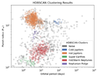
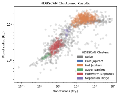
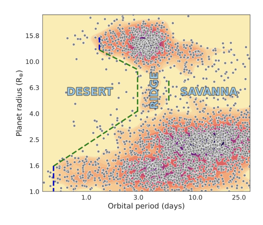
The clustering result is shown in Figures 3 and 4. The clustering method classifies exoplanets into 5 groups, excluding the noise points. We have labeled each group with the classification group names already in use by astronomers. We notice that the HDBSCAN method can successfully identify the largest groups, including Hot/Cold Jupiters, and Neptunes/Super Earths. Surprisingly, the Neptunian Ridge planets are revealed as purple points. This is a recent discovery by Carlos et al., 2024 [6], as shown in Figure 5. These Neptune ridge planets are not Hot Jupiters nor normal Neptunes. People are suggesting that they are Neptune-sized planets that experienced high eccentricity migration.

In Figure 3, we can better understand how HDBSCAN classified those planets. Figure 4 is plotted based on planet radius and planet mass, therefore demonstrating planet interior properties. The slope changes for different clusters, indicating that they have different mass-to-radius relations. This different M to R relation differentiates rocky planets (super earths) from Neptune-sized and Jupiter-sized planets.

The Silhouette Coefficient without the noise points is 0.461, and with noise points is 0.082. The density-based cross-validation (DBCV) gives -0.171. This is expected as exoplanets have a wide and noisy distribution. The most important information we obtained from the classification algorithm is that it has the potential to discover new groups of exoplanets. More detailed investigation into subgroups would require including more features, which will be challenging as more features mean we will have fewer rows and clusters will be more sparse, thus difficult to classify. Therefore, we do not plan to do more experiments on using the unsupervised learning model on the Exoplanet Archive data. We will start testing the unsupervised learning model on the new light curve data from the Kepler dataset, which will be discussed in the Next Steps section.

Next Steps

In our next step, we first plan to implement the Random Forest model and evaluate how well it performs compared to our current results from other models, as well as existing research. After cleaning the dataset, features will be selected based on their significance, which is an estimation with physics knowledge. The data is then split into train and test datasets. The random tree forest model is first turned over a broad hyperparameter space, such as 600 random combinations, to first identify a rough range of good-performance parameters. It was then fine-tuned with the discovered parameters to find maximum accuracy.

More importantly, we plan to use the light curve data from the Kepler dataset. The reason for including the light curve data is that they keep all the raw planet transit information that the Kepler Object of Interest table does not fully keep. We will begin with data preprocessing, select the light curve data with fixed cadence, and slice them into 500-point segments with the deepest transit signal in the center. The labels are the same, which are “Candidate” or “False positive” for each row. We will then use our HDBSCAN model to test on the light curve data, after using PCA to reduce the parameters. This will give us a good intuition of how the data is structured.

Then, we plan to combine both the Kepler table data, which contains information from the planet, star, and also physical models used for fitting the parameters, and the raw information from the light curve, to train a supervised model for better identifying false positives. We will use neural networks for the training, start with CNN, and include transformers if necessary. We will test whether neural networks will give us higher accuracy and precision. Moreover, we will also test our neural network model on other datasets, including the TESS light curve data, to see if our model can migrate to other datasets without much data preprocessing. If we can achieve good results in the TESS dataset, then this will be a remarkable discovery.

Gantt Chart

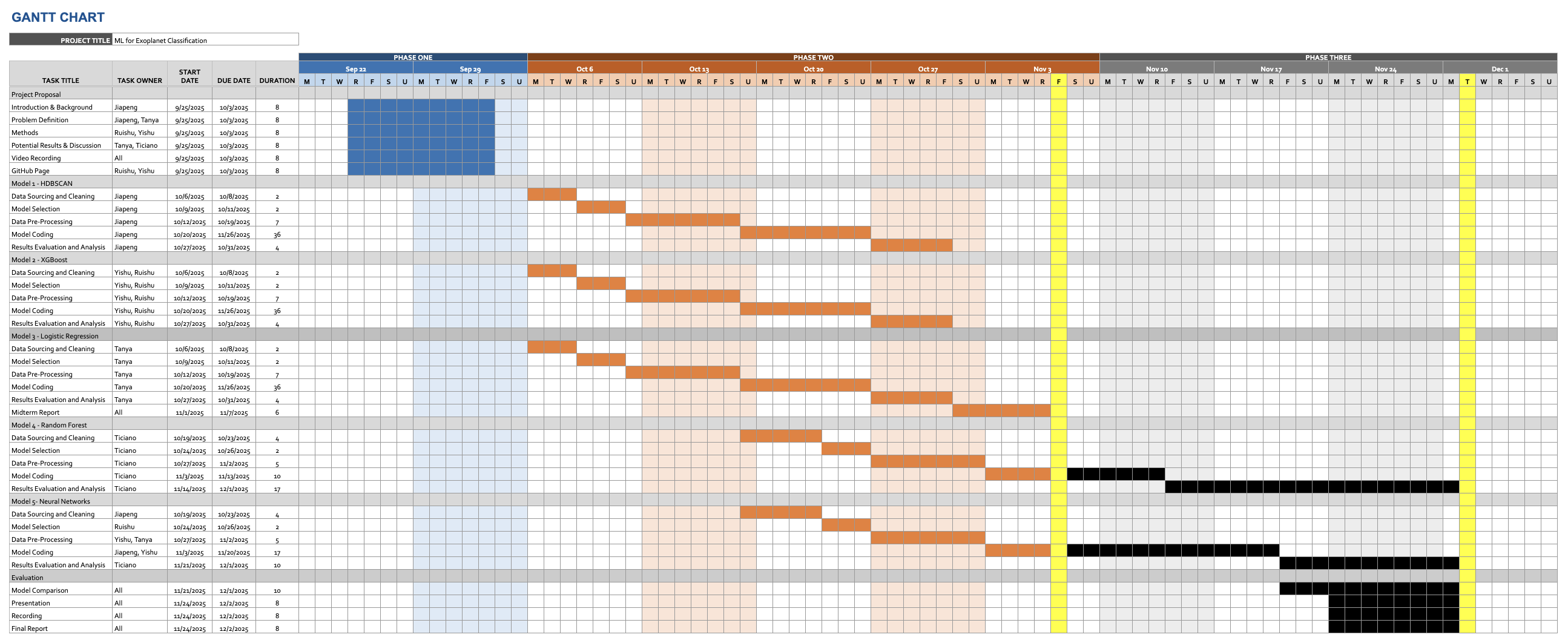
📊 View Detailed Gantt Chart

Contribution Table

Name	Midterm Contributions
Jiapeng Gao	Unsupervised learning: HDBSCAN. Report writing and reviewing.
Ruishu Cao	Supervised learning: XGBoost. Report writing. GitHub Pages.
Tanya Chauhan	Supervised learning: Logistic Regression. Report writing.
Melvin Ticiano Gao	Testing supervised learning models, Report writing, and organizing the GitHub repository.
Yishu Ji	Supervised learning: XGBoost. Report writing. GitHub Pages.

References

• [1] Mayor, Michel, and Didier Queloz. "A Jupiter-mass companion to a solar-type star." nature 378.6555 (1995): 355-359.
• [2] Christiansen, Jessie L., et al. "The NASA Exoplanet Archive and Exoplanet Follow-up Observing Program: Data, Tools, and Usage." arXiv preprint arXiv:2506.03299 (2025).
• [3] Choudhary, Anupma, et al. "Exoplanet Classification through Vision Transformers with Temporal Image Analysis." arXiv preprint arXiv:2506.16597 (2025).
• [4] Rafaih, Ayan Bin, and Zachary Murray. "Detecting False Positives With Derived Planetary Parameters: Experimenting with the KEPLER Dataset." arXiv preprint arXiv:2508.13801 (2025).
• [5] L. McInnes, J. Healy, S. Astels, hdbscan: Hierarchical density based clustering In: Journal of Open Source Software, The Open Journal, volume 2, number 11. 2017
• [6] Castro-González, A., et al. "Mapping the exo-Neptunian landscape-A ridge between the desert and savanna." Astronomy & Astrophysics 689 (2024): A250.